Dual-Stage 3D Printing
A research project applying dual stage control to 3D printing.
An Overview:
As a part of Widener University’s summer research program, I joined a project under Dr. William Nagel working to apply dual-stage actuators to 3D printing in an effort to increase print speeds. Printing faster is a core goal of the 3D printing field, allowing each printer to be more productive, but machines quickly run into bandwidth limitations as speed increases. As high speed, an actuator’s precision becomes worse, and the precision of larger actuators will be worse than small ones. For 3D printing, this means that it is difficult to increase speed without switching to lower-range actuators, which would sacrifice working area.
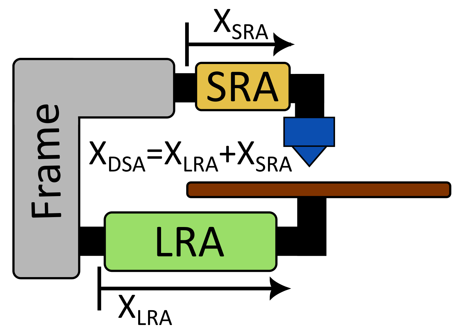
Dual stage systems address this by pairing a large, long rang actuator (LRA) with a smaller one capable of high speed and precision - allowing them to have both range and precision. For the purposes of our 3D printer, the nozzle is mounted to a short-range actuator(SRA) and the bed to the long range actuator(LRA), as illustrated below. However, because each axis now has 2 actuators, controlling it is more complex than a traditional printer. For my research, I focused on designing such a controller.
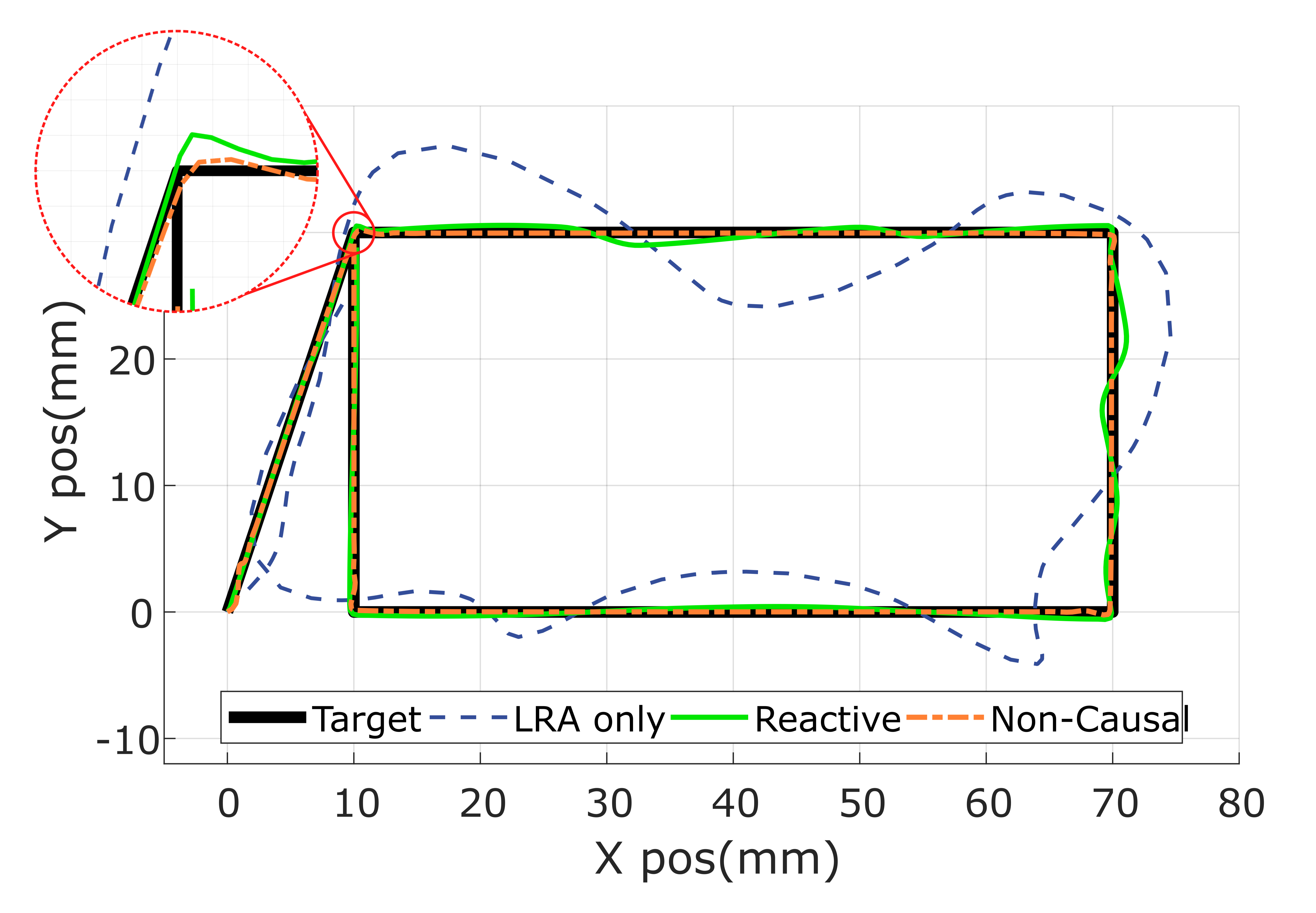
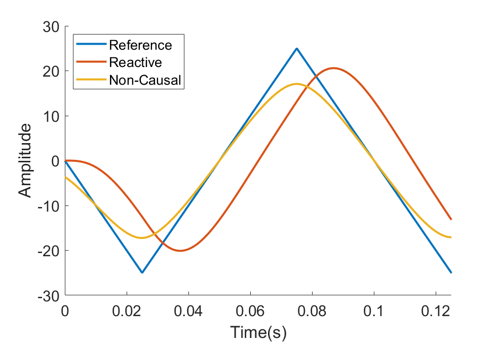
In the final version of the control system(Non-causal controller), the path for each printer axis is generated by parsing standard 3D printing g-code, and then these target trajectories are split into targets for the LRA and SRA, using a low pass filter to separate the lower acceleration motions from the higher-acceleration parts. In previous versions(Reactive controller), the feedback controller received only a single target path for each axis, which it then used to generate commands for the two actuators, but filtering beforehand and separating the control loops improved performance (See implementation details). Below, you can see the final controller compared to this previous, single-loop reactive controller, as well as a reference of how the system would perform without the addition of the short range actuator.
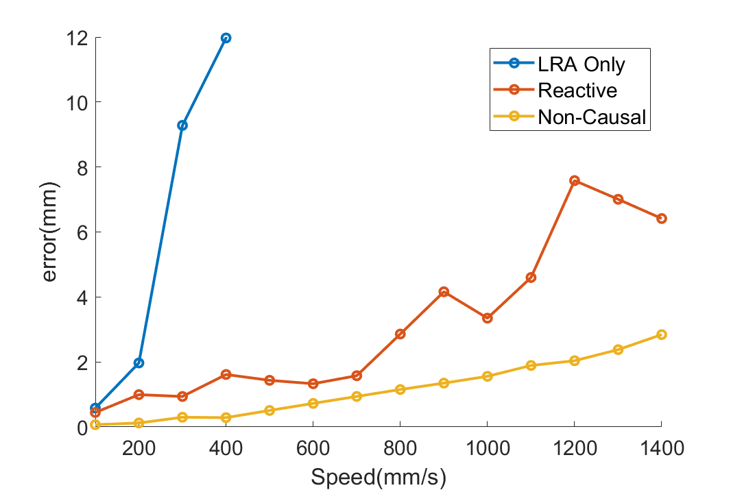
If if instead error is held constant, we can compare the time needed to finish a sample print. Comparing times for each controller where the 98th percentile error is below 1mm resulted in the following print times:
| Printer | Print Time |
|---|---|
| X1 Carbon | 15:29 |
| LRA-only | 37:40 |
| Reactive | 14:41 |
| Non-Causal | 4:55 |
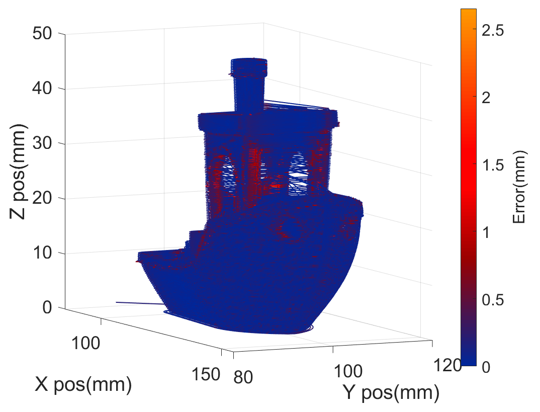
The commercially available Bamboo Labs X1 Carbon is included as a reference, with the time based off testing by Tom’s hardware. A simulation of the test ‘benchy’ print used is also shown below. These simulations show that applying dual-stage control to 3D printing shows promise, and I continue to work on this controller and the printer hardware with the project team. Overall, I learned a huge amount simulation and control, as well as gaining experience in the methodologies used for designing dual-stage systems.
Implementation Details!
The part everyone’s been waiting for: how does this work in practice, and why is this system designed the way it is? At a high level, a 3D model is sliced (using PrusaSlicer), and the g-code this generates is parsed into uniform-time trajectories listing the position of each actuator every millisecond. The X and Y trajectories are then low-pass filtered using a python script to generate LRA and SRA targets for these axes. These target trajectories are used as input to a Simulink model of the dual stage hardware, which is implemented using transfer functions of the dual stage hardware.
The final controller has two key advantages over earlier versions: it uses a non-causal filter on the target trajectories, and separates the control loops for the long and short range actuators. This can be seen generally in the diagram below - showing the control structure for a single dual stage axis. The definitions for each system block are described under System Models.
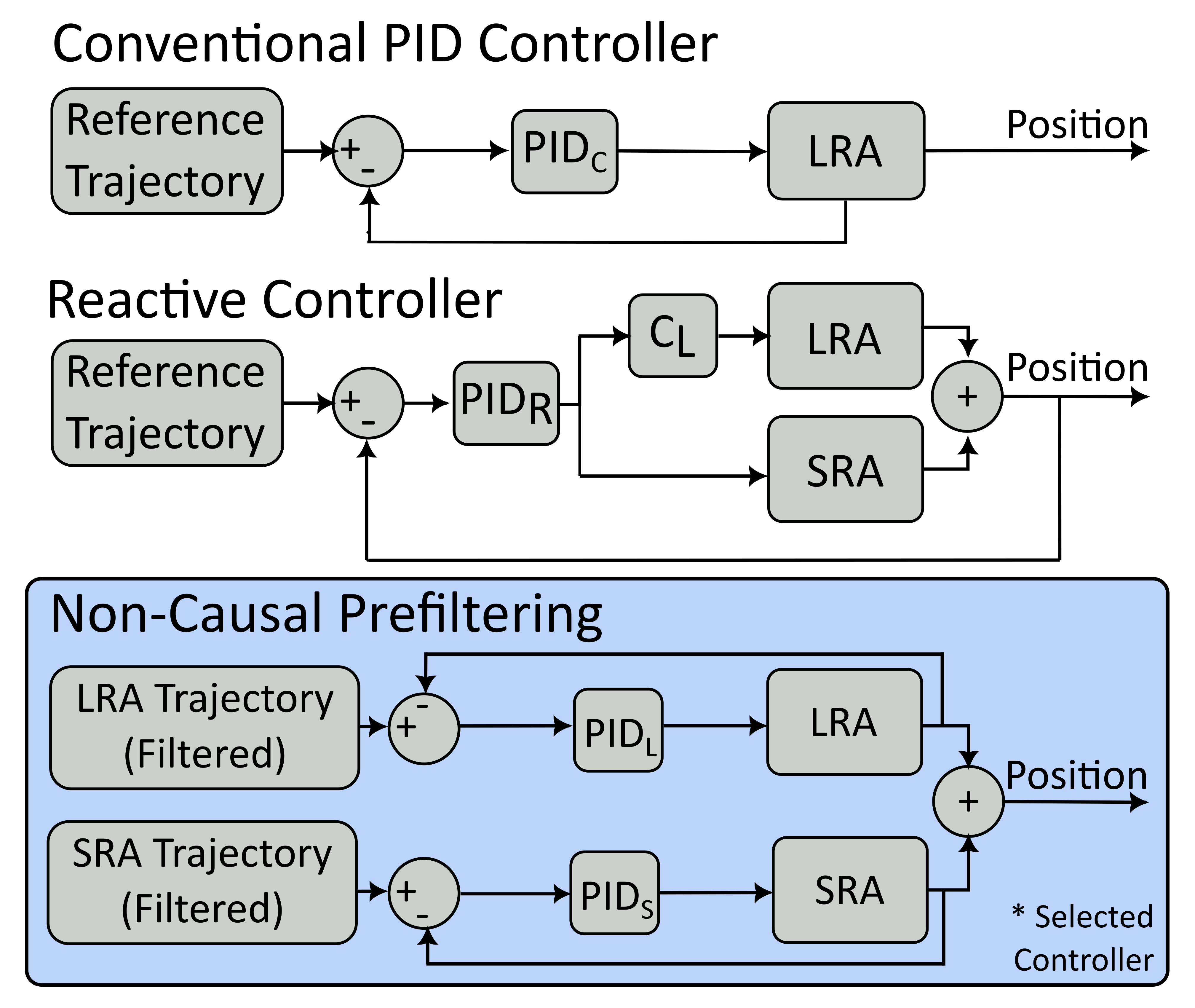
A standard low-pass filter removes the higher frequency components of a signal, which can be thought of as ‘smoothing’ it, but introduces some delay. This is the approach used by the reactive controller - where filtering takes place in the control loop. However, since the entire target path of the actuator is known, a non-causal filter can be used, meaning the filter accounts future target positions to calculate the current smoothed target, and removes the delaying effect. In practice, I used an iterative first order low pass filter of the form \(y[n]=(1-\alpha)*y[n-1]+\alpha*x[n]\), where \(y[n]\) is the output at time \(n\) and \(x[n]\) is the input.
Running this first over filter over the target path forwards and then in reverse results in a second order filtered signal without the time delay introduced by causal filtering. When run over a time-reversed signal, the output depends on input values later in the trajectory, which is only possible because the input is known for all time. Removing the signal lag reduces the LRA error, allowing the system to be more accurate in its movement. In this controller, the SRA is assigned the difference between the original target and the low-pass filtered LRA target.
Switching to two parallel feedback controllers also contributes to improved system performance, also making it much less sensitive to changes in PID tunings, speeding development. In the reactive controller, slight changes in the tuning parameters could cause significant oscillations in the output, but with separate feedback loops each PID controller can be tuned for their specific actuator, improving performance. It made sense to implement these two changes simultaneously, since the non-causal filtering requires having separate inputs to the LRA and SRA controllers and therefore separate control loops, however this makes it difficult to determine how much of the performance improvements can be attributed to each of these changes.
System Models:
For those interested, these are the transfer functions modeling the behavior of our printer as well as the PID controller and filters used in the simulation. \(LRA(s)\) and \(SRA(s)\) model the response of each actuator to an input, and \(PID_j\) represents a standard PID controller in the form of a transfer function. \(C_L\) is a first order low-pass filter, used to filter the PID output in the reactive controller.
\[𝑃𝐼𝐷_𝑗(𝑠)=𝑘_{𝑝_𝑗}+\frac{𝑘_{𝑖_𝑗}}{𝑠}+𝑘_{𝑑_𝑗}𝑠\] \[𝐶_𝐿(𝑠)=\frac{\omega_𝑐}{𝑠+\omega_𝑐}\] \[𝐿𝑅𝐴(𝑠)=𝑘_𝐿\frac{\omega_𝐿^2}{𝑠^2+2\zeta_𝐿 \omega_𝐿 𝑠+\omega_𝐿^2}\] \[𝑆𝑅𝐴(𝑠)=𝑘_𝑠\frac{𝜔_𝑠^2}{𝑠^2+2\zeta_𝑠 \omega_𝑠 𝑠+\omega_𝑠^2}*\frac{𝑠+𝑧}{𝑠+𝑝}\]Where:
\[\omega_c=18Hz\]| Variable: | \(PID_C\) | \(PID_R\) | \(PID_L\) | \(PID_S\) |
|---|---|---|---|---|
| \(k_p\) | 320 | 4.2 | 320 | 175 |
| \(k_i\) | 400 | 770 | 400 | 700 |
| \(k_d\) | 0.2 | 0.28 | 0.2 | 0.455 |